误差反向传播法
用到的知识:
- 计算图进行局部运算
- 简单层的实现
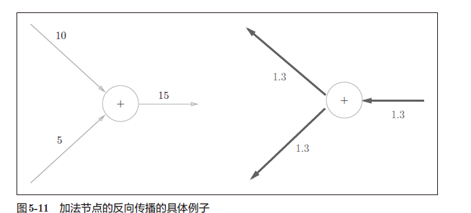
- 加法层
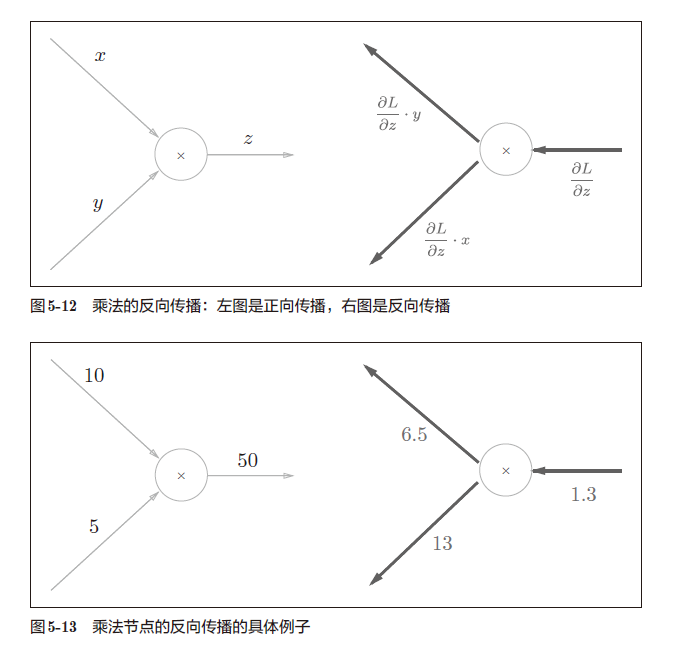
- 乘法层
- 激活函数层的实现
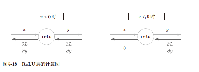
- Relu层
- Sigmoid层
- Affine/Softmax层的实现
跳过计算图介绍
简单层的实现
加法层
python实现
1 | class AddLayer: |
乘法层
python实现:
1 | class MulLayer: |
激活函数层的实现
ReLu层
1 | # 这里输入层都是以numpy数组输入 |
Sigmoid层
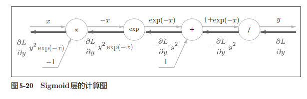

根据以上式子,相应的python实现为:
1 | class Sigmoid: |
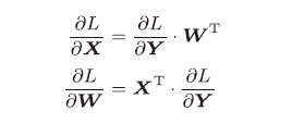
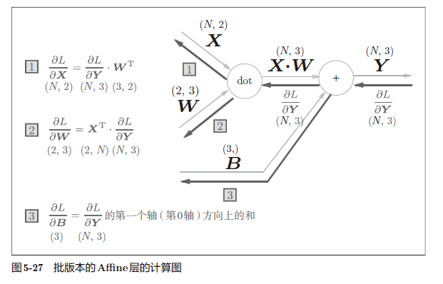
Affine/Softmax层的实现
Affine层的批量化
python实现:
1 | class Affine: |
Softmax-with-loss层
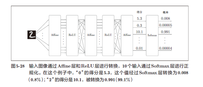
神经网络中进行的处理有推理(inference)和学习两个阶段。神经网络的推理通常不使用Softmax 层。比如,用图5-28 的网络进行推理时,会将最后一个Affine 层的输出作为识别结果。神经网络中未被正规化的输出结果(图5-28 中Softmax 层前面的Affine 层的输出)有时被称为“得分”。也就是说,当神经网络的推理只需要给出一个答案的情况下,因为此时只对得分最大值感兴趣,所以不需要Softmax 层。不过,神经网络的学习阶段则需要Softmax层。
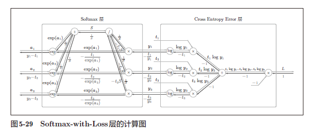
化简计算图可以得到以下的简化图:
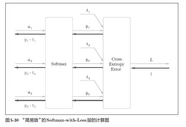
Softmax 层的反向传播得到了(y1 − t1, y2 − t2, y3 − t3)这样“漂亮”的结果。由于(y1, y2, y3)是Softmax 层的输出,(t1, t2, t3)是监督数据,所以(y1 − t1, y2 − t2, y3 − t3)是Softmax 层的输出和教师标签的差分。神经网络的反向传播会把这个差分表示的误差传递给前面的层,这是神经网络学习中的重要性质。刚刚的(y1 − t1, y2 − t2, y3 − t3)正是Softmax层的输出与教师标签的差,直截了当地表示了当前神经网络的输出与教师标签的误差。
这里考虑一个具体的例子,比如思考教师标签是(0, 1, 0),Softmax 层的输出是(0.3, 0.2, 0.5) 的情形。因为正确解标签处的概率是0.2(20%),这个时候的神经网络未能进行正确的识别。此时,Softmax 层的反向传播传递的是(0.3, −0.8, 0.5) 这样一个大的误差。因为这个大的误差会向前面的层传播,所以Softmax层前面的层会从这个大的误差中学习到“大”的内容。
使用交叉熵误差作为softmax 函数的损失函数后,反向传播得到(y1 − t1, y2 − t2, y3 − t3)这样“ 漂亮”的结果。实际上,这样“漂亮”的结果并不是偶然的,而是为了得到这样的结果,特意设计了交叉熵误差函数。回归问题中输出层使用“恒等函数”,损失函数使用“平方和误差”,也是出于同样的理由(3.5 节)。也就是说,使用“平方和误差”作为“恒等函数”的损失函数,反向传播才能得到(y1 −t1, y2 − t2, y3 − t3)这样“漂亮”的结果。
交叉熵误差函数python实现:
1 | def cross_entropy_error(y,t): |
Softmax-with-Loss 层的实现
1 | def softmax(x): |
误差反向传播法的实现
神经网络学习的全貌图
前提
- 神经网络中有合适的权重和偏置,调整权重和偏置以便拟合训练数据的过程称为学习。神经网络的学习分为下面4 个步骤。
步骤1(mini-batch)
从训练数据中随机选择一部分数据。
步骤2(计算梯度)
计算损失函数关于各个权重参数的梯度。
步骤3(更新参数)
将权重参数沿梯度方向进行微小的更新。
步骤4(重复)
- 重复步骤1、步骤2、步骤3。
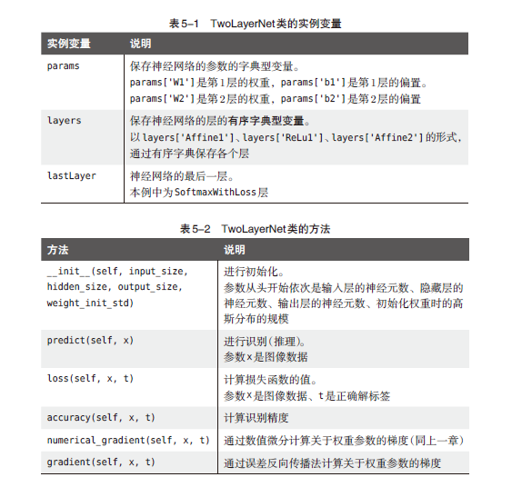
基于BP算法的TwoLayerNet的实现
1 | import numpy as np |
梯度确认
数值微分的优点是实现简单,因此,一般情况下不太容易出错。而误差反向传播法的实现很复杂,容易出错。所以,经常会比较数值微分的结果和误差反向传播法的结果,以确认误差反向传播法的实现是否正确。确认数值微分求出的梯度结果和误差反向传播法求出的结果是否一致(严格地讲,是非常相近)的操作称为梯度确认(gradient check)。
1 | # coding: utf-8 |
神经网络学习(bp算法版)
1 | import sys, os |


