关于axis轴参数理解
坐标轴
假定是二维元素
就是行元素和列元素变化的方向
axis=1对列进行操作,axis=0对行进行操作
tf.Tensor
- list
- np.array
- tf.Tensor
为了实现gpu加速,所以重新开发了科学计算库
基本类型
- scalar: 1.1
- vector:[1.1,2.2,3.3]
- matrix:[[1.1,2.2],[3.3,4.4]]
- Tensor:dim>2
在 TensorFlow 中间,为了表达方便,一般把标量、向量、矩阵也统称为张量,不作区分,需要根据张量的维度数或形状自行判断
int,float,double
int32,int64,float32,float64
bool
string
tf.constant()
用来创建一个标量
可以用以下方法:
- .gpu( ) :使用gpu
- .cpu( ) :使用cpu
- .numpy( ) :返回当前值的numpy的数据类型
- .nidm : 返回维度
- .shape :返回形状
tf.rank( ) :
可以用来查看张量对象的所有信息
tf.is_tensor( ):
用来判断是否是tf.tensor类型
tf.convert_to_tensor( ):
可以把numpy类型转化为tensor类型
tf.cast(x,dtype=)
可以转化类型的精度
tf.Variable
创建一个待优化张量
由于梯度运算会消耗大量的计算资源,而且会自动更新相关参数,对于不需要的优化的张量,如神经网络的输入𝑿,不需要通过tf.Variable 封装;相反,对于需要计算梯度并优化的张量,如神经网络层的𝑾和𝒃,需要通过tf.Variable 包裹以便TensorFlow 跟踪相关梯度信息。
比起普通张量多了两个属性【对象属性】:
name
name 属性用于命名计算图中的变量,这套命名体系是TensorFlow 内部维护的,一般不需要用户关注name 属性
trainable
trainable属性表征当前张量是否需要被优化,创建Variable 对象时是默认启用优化标志,可以设置
trainable=False 来设置张量不需要优化。
然而普通张量其实也可以通过GradientTape.watch()方法临时加入跟踪梯度信息的列表,从而支持自动求导功能。
创建一个tensor
转换numpy类型
tf.constant( ) 或 tf.Varible( ) 或 tf.convert_to_tensor( )
可以使用这三个函数来转化numpy类型来创建tensor
1 | tf.convert_to_tensor(np.ones([2,3]),dtype=tf.float32) |
全部初始化为指定值
tf.zeros( )
创建全0张量
tf.zeros([ ])
传入[1,2]类似np.zeros((1,2))或np.zeros([1,2])
tf.zeros_like( )
与np.zeros_like( )类似
tf.ones( )
创建全1 张量
使用方法同上
tf.ones_like( )
使用方法同上
tf.fill(shape,value)
除了初始化为全0,或全1 的张量之外,有时也需要全部初始化为某个自定义数值的
张量,比如将张量的数值全部初始化为−1等。
1 | tf.fill([2,2],3) |
创建已知分布的张量
正态分布
tf.random.normal(shape, mean=0.0, stddev=1.0)
可以创建形状为shape,均值为mean,标准差为stddev 的正态分布𝒩($mean, stddev^2$)。
tf.random.truncated_normal(shape, mean=0.0, stddev=1.0)
会截取正态分布的一部分,有利于sigmoid函数的梯度下降
1 | tf.random.truncated_normal([3,3], mean=0.0, stddev=1.0) |
均匀分布
tf.random.uniform(shape, minval=0, maxval=None, dtype=tf.float32)
可以创建采样自[minval, maxval)区间的均匀分布的张量。
- 如果需要均匀采样整形类型的数据,必须指定采样区间的最大值maxval 参数,同时指定数据类型为tf.int*型
1 | tf.random.uniform([3,3],minval=1,maxval=100) |
创造序列
tf.range(limit,delta=1)
tf.range(limit, delta=1)可以创建[0, limit)之间,步长为delta 的整型序列,不包含limit 本身。
Scalar:
- [ ]
- loss
- accuracy
Vector:
- Bias
- [out_dim]
Matrix:
- input x:[b,vec_dim]
- weight:[input_dim,output_dim]
Dim=3 Tensor:
- x: [b,seq_len,word_dim]
一般将单词通过嵌入层(Embedding Layer)编码为固定长度的向量,比如“a”编码为某个长度3 的向量,那么2 个等长(单词数量为5)的句子序列可以表示为shape 为[2,5,3]的3 维张量,其中2 表示句子个数,5 表示单词数量,3 表示单词向量的长度。
Dim=4 Tensor
- Image:[b,h,w,3]
- feature maps:[b,h,w,c]
图片相关的处理
Dim=5 Tensor
- Single task: [b,h,w,3]
- meta-learning: [task_b,b,h,w,3]
索引与切片
Basic indexing and Numpy-style indexing
在 TensorFlow 中,支持基本的[𝑖],[𝑗] ⋯标准索引方式,也支持通过逗号分隔索引号的索引方式。
推荐用x[1,2,3]这种索引方式
1 | x=tf.random.normal([1,2,3,4],mean=0,stddev=1) |
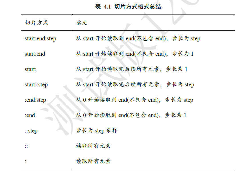
start : end :step
与numpy中使用方式相同
为了避免出现像 [: , : , : ,1]这样过多冒号的情况,可以使用⋯符号表示取多个维度上所有的数据,其中维度的数量需根据规则自动推断:当切片方式出现⋯符号时,⋯符号左边的维度将自动对齐到最左边,⋯符号右边的维度将自动对齐到最右边,此时系统再自动推断⋯符号代表的维度数量
读取第 1~2 张图片的G/B 通道数据,实现如下:
1
x[0:2,...,1:]

特别地,step 可以为负数,考虑最特殊的一种例子,当step = −1时,start: end: −1表示从start 开始,逆序读取至end 结束(不包含end),索引号𝑒𝑛𝑑 ≤ 𝑠𝑡𝑎𝑟𝑡。考虑一个0~9 的简单序列向量,逆序取到第1 号元素,不包含第1 号
Selective Indexing
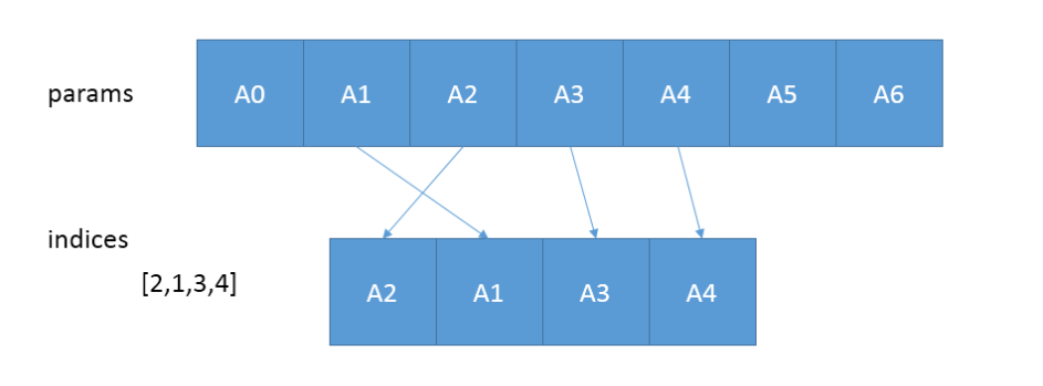
tf.gather(params,indices,axis=0)
从params的axis维根据indices的参数值顺序获取切片
只在一个维度中取值
tf.gather_nd( params, indices, name=None )
这里的idices可以为[[0, 2], [0, 4], [2, 2]]或[[0], [1]]或([0])或[0, 1]
类似坐标轴取数
有一点不同的地方是[[2,3]]和[2,3]一个返回向量,一个返回标量
tf.boolean_mask( tensor, mask, name=’boolean_mask’, axis=None )
根据bool类型mask数组来判断是非保留数据
1
2
3
4
5import tensorflow as tf
a=tf.range(5*5*5*5)
a=tf.reshape(a,[5,5,5,5])
tf.boolean_mask(a,mask=[True,True,False,False,True])#只取0,1,4号第0轴元素
tf.boolean_mask(a,mask=[True,True,False,False,True],axis=3)#只取第3轴的0,1,4号
维度变换
全连接层的向前传播:
在tensorflow中:$Y=X@W+b$
其实都差不多
tf.reshape(x, new_shape)
通过tf.reshape(x, new_shape),可以将张量的视图任意地合法改变
tf.expand_dims(x,axis) 和 tf.squeeze(x,axis)
tf.expand_dims(x, axis)可在指定的axis 轴前可以插入一个新的维度
需要注意的是,tf.expand_dims 的axis 为正时,表示在当前维度之前插入一个新维度;为
负时,表示当前维度之后插入一个新的维度。tf.squeeze(x,axis)可删除指定轴
tf.transpose(x,perm)
perm提供新的轴的读取顺序
广播
tf.broadcast_to( input, shape, name=None )
几乎不会用到,tensorflow里有与numpy类似的广播机制
将原始矩阵成倍增加
基本运算
Outline
+-*/
** , pow ,square
sqrt
//,%
exp,log
tf.math.log #只以e为底
其他底只能通过对数相除得到
tf.exp
tf2.2 exp已经被移到math模块
@,matmul
类似np.dot
linear layer
Operation type
element-wise(对应元素运算)
- +-*/
matrix-wise
- @,matmul
- dim-wise
- reduce_mean/max/min/sum
前向传播实战
与python+numpy实现方式类似,但tensorflow提供了自动求导函数
1 | #!/usr/bin/env python |
有几个注意事项:
tf.GradientTape( )默认只监控由tf.Variable创建的traiable=True属性(默认)的变量:
常用语句:
with tf.GradientTape( ) as tipe:
tipe.gradient(f,[value])
对f( value )求导
tf.data.Dataset.from_tensor_slices((x,y)).batch(128)
- tf.data.Dataset.from_tensor_slices( )会对最外层分割成单独元素,第0轴
- .batch( )方法可以重新将单独元素打包
.assign_sub( )方法可以实现tf.Variable创建的变量的自我更新
因为如果使用w=w-lr*grads , 经过减法运算后的返回值为tf.tensor , 不为tf.Variable ,会影响下一次循环
进阶操作
数据打乱
tf.random.shuffle(x)
将x中元素顺序打乱
合并与分割
合并
tf.concat([,],axis)
按对应轴合并数据
1 | import tensorflow as tf |
tf.stack([,],axis)
可在指定的axis 轴前可以插入一个新的维度,并合并传入的数据
但对合并数据shape有要求,必须保持一致的shape
分割
tf.unstack([,],axis)
可以按轴拆开数据
tf.split(x,num_or_size_splits,axis)
x 参数:待分割张量。
num_or_size_splits 参数:切割方案。当num_or_size_splits 为单个数值时,如10,表
示等长切割为10 份;当num_or_size_splits 为List 时,List 的每个元素表示每份的长
度,如[2,4,2,2]表示切割为4 份,每份的长度依次是2、4、2、2。axis 参数:指定分割的维度索引号。
数据统计
向量范数
tf.norm(x,ord,axis)
在 TensorFlow 中,可以通过tf.norm(x, ord)求解张量的L1、L2、∞等范数,其中参数
ord 指定为1、2 时计算L1、L2 范数,指定为np.inf 时计算∞ −范数。
最值,均值,和
以下函数在没指定axis的值时,默认在所有维度进行判断
tf.reduce_max(x,axis)
求最大值
tf.reduce_min(x,axis)
求最小值
tf.reduce_mean(x,axis)
求均值
tf.reduce_sum(x,axis)
求和
tf.argmax(x,axis) 和 tf.argmin(x,axis)
与numpy中使用方式一致,返回索引
张量比较
tf.equal(a,b) 和 tf.math.equal(a,b)
可以将预测值与真实值比较,返回布尔类型的张量
tf.unique(x)
返回x的不充分表 和 原来表与不重复表中的索引
1 | a=tf.constant([3,4,4,1,1,1,0]) |
可以使用tf.gather(Unique,idx)完成逆运算
张量排序
Outline:
- sort/argsort
- Topk
- Top-5 Acc.
tf.sort(x,direction=’ASCENDING’) 和 tf.argsort(x,direction=’ASCENDING’)
tf.sort( )按照升序或者降序对张量进行排序
tf.argsort( )按照升序或者降序对张量进行排序,但返回的是索引direction=’DESCENDING’ 时为降序
direction=’ASCENDING’ 时为升序
tf.math.top_k(x,k)
tf.math.top_k(x,k)返回带有前k个最大值的对象
如a=tf.math.top_k(x,k)
- a.value为带有前k个最大值的张量
- a.indices为带有前k个最大值的索引的张量
应用:
- top-k accuracy:
- Prob:[0.1,0.2,0.3,0.4]
- Label:[2]
Only consider top-1 prediction: [3] 0%
Only consider top-2 prediction: [3,2] 100%
Only consider top-3 prediction: [3,2,1] 100%
一般会考虑top-5 的预测值去判断模型的性能好坏
Top-k Accuracy: 【仅限二维】
1 | def accuracy(output,target,topk=(1,)): |
accuracy(output,target,topk=(1,2,3,4,5))
填充与复制
Outline
- pad
- tile
- broadcast_to
tf.pad( tensor,paddings,mode=’CONSTANT’,name=None )
- tensor是待填充的张量
- paddings指出要给tensor的哪个维度进行填充,以及填充方式,要注意的是paddings的rank必须和tensor的rank相同
- mode指出用什么进行填充,’CONSTANT’表示用0进行填充(总共有三种填充方式,本文用CONSTANT予以说明pad函数功能)
- name就是这个节点的名字
padding=([[ , ],[ , ],[ , ]])
padding的输入大概为这种格式,一个列表表示一个维度的上下左右填充数目且一个列表只有两个元素,表示作用
1 | a=tf.ones([3,3]) |
tf.tile(tensor,[ , ,])
[ , , ]在里面填每个维度有多少的基础单元tensor,因为必有一个基础单元,所以不能填0
1 | a=tf.constant([[1,2,3],[3,4,5]]) |
tf.broadcast_to(tensor,[ , , ])
把tensor尽可能填充成shape[ , , ]
张量限幅
tf.maximum(tensor,x) 和 tf.minimum(tensor,x)
用法同numpy
tf.clip_by_value(a,min,max)
用法相当于minimum(max,maximum(min,a))
将数据输出限定到一个闭区间内
tf.clip_by_norm(a,number)
将向量先变成单位向量再乘以number的值,相当于改变向量的模长,不会改变梯度的方向
tf.clip_by_global_norm(grads,number)
new_grads,total_norm = tf.clip_by_global_norm(grads,number)
梯度裁断(Gradient Clipping)有利于解决梯度爆炸和梯度消失
高阶操作技巧
Outline:
- Where
- scatter_nd
- mashgrid
tf.where
通过 tf.where(cond, a, b)操作可以根据cond 条件的真假从参数𝑨或𝑩中读取数据,条件
判定规则如下:其中𝑖为张量的元素索引,返回的张量大小与𝑨和𝑩一致,当对应位置的cond𝑖为True,𝑜𝑖从
𝑎𝑖中复制数据;当对应位置的cond𝑖为False,𝑜𝑖从𝑏𝑖中复制数据。
但是只传入一个参数时,如tf.where(tensor),会返回非零元素的索引值所构成的tensor
tf.scatter_nd(indices,updates,shape)
通过 tf.scatter_nd(indices, updates, shape)函数可以高效地刷新张量的部分数据,但是这
个函数只能在全0 的白板张量上面执行刷新操作,因此可能需要结合其它操作来实现现有
张量的数据刷新功能
1 | In [62]: # 构造写入位置,即2 个位置 |
tf.meshgrid(x,y)
与matlab里的meshgrid用途和操作一致
数据加载(tenserflow预设数据集)
Outlline
- keras.datasets
- boston housing
- mnist/fashion-MNIST dataset
- cifar10/100
- imdb
- tf.data.Dataset.from_tensor_slices
- shuffle
- map
- batch
- repeat
常用函数
(x,y),(x_test,y_test)=tf.keras.datasets.mnist.load_data( )
tf.one_hot(tensor,depth= )
db=tf.data.Dataset.from_tensor_slices((x_test,y_test))
.shuffle(number)方法
打乱顺序
.map( )方法
数据预处理
1
2
3
4
5
6def prepocess(x,y):
x=tf.cast(x,dtype=tf.float32)/255
y=tf.cast(y,dtype=tf.int64)/255
y=tf.one_hot(y,depth=10)
return x,y
db2=db.map(prepocess).batch( )方法
.repeat( )方法
1
2
3db4=db.repeat(30)
for x,y in db4:
pass数据加载
1 | def prepocess(x,y): |
测试张量
1 | #!/usr/bin/env python |


